Welcome to the second part of the terrain engine series (The first part can be found here). This article focuses on the basic generation formalism for our terrain. Actual generation of huge worlds will be covered in a different series.

Volume Chunks

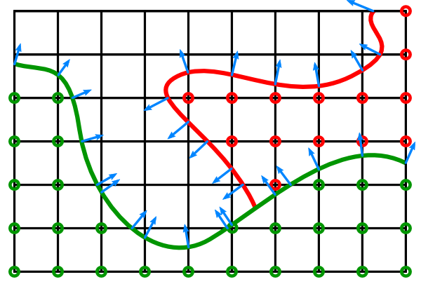
The terrain data that we want to generate is called Hermite Data. As introduced in the last article, this data consists of material indices at grid points and $$(n_x, n_y, n_z, t)~$$ at edges that inhibit a material change. $$(n_x, n_y, n_z)~$$ describes the normal of the isosurface (i.e. our terrain mesh) and $$t~$$ the relative position where the surface intersects with the grid edge. Generating this data is a little bit more involved than your usual density-based Marching Cubes data but the reward is a lot of fine control over the terrain shape. An example of such volume data for two different materials (red and green) is shown below. Normals are indicated in blue.

To make processing an infinite world feasible, a chunk notation is introduced. A chunk is a cubical block of Hermite Data that represents a region of the world at a fixed resolution. Chunks are always axis-aligned (i.e. their regions are defined by AABBs) and managed in a hierarchical manner. The next part of this series will describe this hierarchy in detail, including its application to implement level-of-detail (LOD).

A little more terminology: Chunks have a resolution $$n~$$ resulting in $$(n+1)^3~$$ material indices and $$3 \cdot (n+1)^2 \cdot n~$$ edges. The effective resolution of a chunk is the distance between two neighboring grid points in global coordinates (i.e. a $$16^3~$$ chunk with a region of $$[1,5]^3~$$ has a resolution of $$16~$$ but an effective resolution of $$0.25 = \frac{4}{16}~$$). Choosing $$(n+1)^3~$$ material indices for power-of-two values $$n~$$ is beneficial for LOD-calculations (cf. next article).

The whole generation problem can now be condensed to: Generate a volume chunk that represents terrain.

CSG Tree

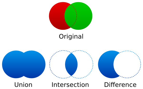
To make this generation more intuitive and expressive, a CSG notation is used. Originally, constructive solid geometry (CSG) is used for modelling with sets. For example, given two objects $$A~$$ and $$B~$$, we could formulate their union as $$A \cup B~$$, their intersection as $$A \cap B~$$, or "A without B" as $$A \setminus B~$$. This can be translated to density functions $$f~$$ and $$g~$$ where $$\overline{A}~$$ translates to $$-f~$$, $$A \cup B~$$ to $$\mathrm{min}(f, g)~$$, $$A \cap B~$$ to $$\mathrm{max}(f, g)~$$, and $$A \setminus B~$$ to $$\mathrm{max}(f, -g)~$$ (assuming $$\lt 0~$$ being "inside" and $$\gt 0~$$ being "air").

If CSG operations can be translated so easily into mathematical formulas, why bother introducing a new formalism for them if our expression system can already handle this? There are three main reasons: First, if $$A~$$ and $$B~$$ represent different materials, this information would be lost if compressed into one density formula. The second reason is that the resulting formulas are getting quite complex, difficult to read, and hard to maintain. The last reason is less obvious and concerns terrain modification ("construction", "destruction"). Most operations that modify the terrain can be modeled as a CSG operation. For example, digging can be implemented by $$T \setminus D~$$ where $$T~$$ is our current terrain and $$D~$$ the shape that we dig out. Thus, for any operation on the terrain, we could simply append this operation to our formula and reevaluate all chunks that are affected (assuming we can specify some kind of bounding volume to which the operation is restricted). After digging the same location a hundred times, the formula would contain a hundred more $$\mathrm{max}~$$ operations. The resulting system would slow down prohibitively in a short amount of time.

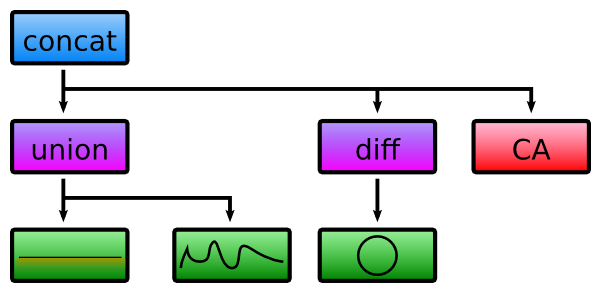
In the CSG tree, each operation is modeled as an operation $$f~$$ that can be seen as $$B \leftarrow f(A)~$$ where $$A~$$ and $$B~$$ are volume chunks and $$B~$$ is the result of $$f~$$ applied to $$A$$. Given a generation function $$g$$, generating the terrain $$T~$$ is just $$T \leftarrow g(\emptyset)~$$ (where $$\emptyset~$$ is an all-air chunk). All operations are ordered and terrain modifications can simply be appended at the back of the CSG "queue". While it is not a tree in a mathematical sense (trees are not ordered), it can be represented as such to improve readability. The following tree is an example of a CSG tree that first combines a sand plane with some mountains (union node), then subtracts a sphere shape (diff node) and finally applies a cellular automata that adds a grass layer (CA node). The exact meaning of these nodes are explained in later sections.

This formulation has a lot of advantages. As an operation operates on a complete volume chunk it is free to modify it in any way, making each operation quite cache-friendly and therefore efficient. The current terrain has the correct format to qualify as input data and can be directly overwritten by the output of an operation. Therefore, a terrain modification $$m~$$ can be executed as $$T \leftarrow m(T)~$$ without the need to store all previous operations. A notable benefit is that this allows for modification of non-generated or non-loaded terrain by simply appending a serialized version of the operation to its CSG tree. Also, network synchronization of terrain modification can be done by sending the serialized operation instead of the actual volume data. In most cases, this should result in significantly less amount of data transferred. A more exotic advantage is that if a chunk was generated and its complete CSG tree is known, we could estimate the cost of generating it. With that information we could decide if we really want to store the chunk on the disk or just its CSG tree and generate it again next time, depending on what is deemed cheaper. This could be done even after terrain modification and may prove a very effective way to "compress" the terrain.

The following sections introduce the operations that are implemented or planned.

Basic Operations

There are some operations that don't really generate volume data but combine it to achieve various effects. All these operations have children $$c_1,\dots,c_n~$$ in their CSG nodes.

Concat

The most simple one is concat and models consecutive execution of child operations. It is defined by:

$$\mathrm{concat}(A) = c_n(c_{n-1}(\dots c_2(c_1(A)) \dots ))~$$

A CSG tree itself can be seen as an implicit concat node as "appending an operation" translates to "appending a child to the concat node".

Union, Difference, Intersection

In set notation, the union operation is defined by:

$$\mathrm{union}(A) = A \cup c_1(\emptyset) \cup c_2(\emptyset) \dots \cup c_n(\emptyset)~$$

This means, all children are "generated" (application at $$\emptyset~$$) and then their results are united. The union of two different materials is not well-defined and we therefore define our asymmetric union by letting the second operand dominate (i.e. the right-hand side material has precedence). Also, any edge data of the second operand overwrites the data of the first operand. This last restriction may be somewhat lifted if multiple data sets per edge are allowed but this is not yet supported. Difference and Intersection are defined analogously using $$A \setminus B~$$ and $$A \cap B~$$ with adapted edge and material handling. An example of a CSG operation on Hermite data can be found in the appendix at the end of this article.

Density Function

The first and maybe "traditional" way of actually generating terrain data is implemented by using a density function $$f(x,y,z) \to \mathbb{R}~$$. As stated above, we want to avoid a "full-density" solution but modeling a single-material object (e.g. a rock or a sand plane) can be easier and more intuitive using densities. Combining multiple objects can be done using the previously described basic operations.

So how does Hermite data generation using a density function work? First, we evaluate the function $$f~$$ at all grid points and set the material of that point to our target material if the density is below zero and to air if above zero. As we are only interested in the materials, this step can be sped up by using the range prediction of our expression system (if the lower bound of a region is above zero, the complete region is air, if the upper bound is below zero, the region is full material). We then consider all edges with a material change and execute an adaptive binary search between the two grid points to find the intersection of the isosurface with the edge (i.e. we search for $$f = 0~$$ on the edge). Using a maximum of five steps and a density function that is roughly linear we usually end up at less then $$0.1\%~$$ difference to the actual intersection. In this situation, we have the parameter $$t~$$ and want to calculate the isosurface normal $$n~$$. While we could do this by finite differences, our expression system allows for analytic derivation (i.e. calculating $$\frac{\delta}{\delta v} f~$$ where $$v~$$ is an input variable of $$f~$$). The normal $$n~$$ can then be calculated by normalizing the density gradient $$\nabla f = \left( \frac{\delta}{\delta x} f, \frac{\delta}{\delta y} f, \frac{\delta}{\delta z} f \right)~$$ yielding the real isosurface normal (this is especially useful for hard features).

Normal calculation and binary search (together: intersection calculation) is more expensive than simple density evaluation but is only required at material changes, not for each grid point. A little bit of benchmarking revealed that for normal terrain only $$10\%~$$ to $$20\%~$$ generation time is required for intersection calculation. Also, there is a lot of optimization potential in the expression system for normal generation that has not been realized yet.

Heightmap

While we explicitly chose a 3D representation of the terrain to allow for complex terrain and terrain modification, supporting the simpler heightmaps as a CSG operation has its benefits. Heightmaps are easy to create, to understand, to maintain, and to evaluate. Typical applications are deserts or simple hills.

As any heightmap $$h(x,z)~$$ can be represented as a density function $$f(x,y,z) = y - h(x,z)~$$ (though the normal quality may not be excellent), the heightmap operation is currently not implemented but planned. Normals can be calculated analytically by normalizing $$( \frac{\delta}{\delta x} h ,1, \frac{\delta}{\delta z} h)~$$. Generation from a heightmap is generally faster as we only need to evaluate $$(n+1)^2~$$ values instead of $$(n+1)^3~$$ and then directly "fill" vertical columns of volume data.

Mesh Voxelization

Heightmap and density function based generation is quite mathematical, even for designers. In the case of heightmap generation, this can be alleviated by defining the heightmap through images. However, creating a normal 3D mesh terrain in an established design tool and then using this to define the volume data is a valuable way to generate unique terrain parts that would be hard to achieve by the function-based formalism. Therefore, we support a CSG operation that voxelizes meshes into the volume data. In our current implementation this works by shooting rays along grid edges through the mesh, sort all hit triangles by intersection point and then alternate inside/outside along this ray.

Normals are simply face normals of the triangles (or barycentrically interpolated vertex normals). While this is reasonably fast for smaller meshes, it quickly slows down for vertex-rich ones. We will improve our implementation by hierarchically managing the vertices and introduce several steps of caching.

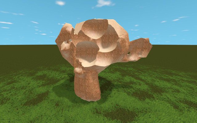
The following image shows a voxelized version of the Blender mascot, Suzanne. Afterwards, it was modified by some diff nodes that had density functions of spheres attached.

Cellular Automata Post-processing

By using the basic operations and the three generation operations, a lot of terrain can already be defined. However, some desirable functions are hard to formulate efficiently. For example, defining a smooth terrain plane with a very rough surface would require high-frequency noise added to a low-frequency plane. The noise must be carefully chosen in order to prevent holes and achieve the rough surface. Another example would be one layer of grass above the earth. This could be designed by placing a grass function and then applying the union operator to the earth function slightly below it. Although these might work, they are neither intuitive nor efficient nor stable. A better way to specify the grass layer would be a post-process that can access the neighboring material indices. In this process, we would then specify: Whenever we find an "air" material with an "earth" material directly below it, convert the "air" to "grass".

This way of thinking is exactly what cellular automata (CA) convey. In the CA formalism, the next state of each cell depends on its current state and the state of all neighbors. A cell of a CA is a grid point with a certain material. The state of a cell consists of the material and the surrounding six edges. Using cellular automata for terrain design was only recently added to our feature list and is therefore neither fully implemented nor tested in detail. However, the potential gain in expressiveness is considerable.

Conclusion

In this article we presented the first formalism for generating the terrain. After introducing the underlying data structure of volume chunks containing Hermite data, the CSG tree concept was introduced. Apart from classic CSG operations (union, difference, intersection), the generation functions based on 3D density functions, 2D heightmaps, or mesh voxelization were presented. For increased expressiveness, terrain post-processing based on cellular automata was sketched.

In the next article, our level-of-detail system with focus on the chunk hierarchy will be described.

Appendix - Hermite CSG Operation

As it is not immediately apparent how CSG operations on Hermite data work, this appendix presents a small example to clarify our implemented behavior. The example has two volume data sets $$A~$$ and $$B$$:

The following images show the two variants of the union operation and a diff operation:

The material indices are trivial to calculate: For $$A \cup B$$, all non-air materials of $$B~$$ override the corresponding material in $$A$$. For $$A \setminus B$$, all non-air materials of $$B~$$ result in air.

Updating the intersection normals is similar. In the case of a union $$A \cup B$$, all intersection normals that matter in $$B~$$ (i.e. they describe a material change in $$B$$) override the data stored in $$A$$. While this can yield slightly imprecise results when more than one intersection per edge is present, this case is not that common and a solution would require considerable overhead. For volume difference, we have a slightly deviant behavior. As this operation models "subtracting" $$B~$$ from $$A$$, intersection normals in $$B~$$ may only override the data in $$A~$$ if the resulting volume data represents a smaller non-air volume. This is the case if the intersection in $$B~$$ lies closer to the non-air material in $$A~$$ than the corresponding intersection in $$A$$. Otherwise, the difference operation could wrongly increase the volume.

While it seems that the stored intersection normals are sometimes oriented in the wrong direction, this actually doesn't matter. The calculated feature points in the Dual Contouring algorithm depend on the quadratic distance to the planes defined by the intersection normals, which is independent of their orientation. When the actual mesh is extracted, all faces can be oriented correctly by considering the materials of the current edge (i.e. the normals can be re-oriented correctly on-the-fly).